Introduction to R: Day 2
September 20, 2017
Outline
- RStudio projects
- “Base” R graphics
- plotting one or two continuous variables
- customizable elements of plots
- saving plots to a file
Create a new project for today
First, let’s see how RStudio projects work in practice. We saw in Part 1 how they let you divide your work into self-contained contexts, since each project has its own working directory, workspace, history, and source documents.
Exercise: Projects
- create a new RStudio project
create a couple of variables and plot them, e.g.:
X <- rnorm(20, 3, 2) Y <- rnorm(20, X/2+2.5, 1.5)- quit RStudio (“yes” to save) and start again.
- switch back to the project we used on Day 1
switch back to today’s project so we can work.
Note the following happens in RStudio when switching to an existing project:
- restore the environment and history
- set the current working directory to the project directory.
- restore documents that were open in the editor tabs
- arrange panels where they were when the project was last open
Environment/workspace
Objects that you create by assignment make up your R workspace. The workspace is shown in the Environment tab in RStudio, and so the term “environment” is sometimes used, even though strictly speaking that’s not [what “environment” means][R-environment] in the R programming language itself. But the meaning is usually clear from the context, and the latter won’t normally be something you have to deal with.
It’s important to remember that the workspace exists only in your computer’s memory: unless you save it to the disk, it will be gone once the R application exits (or you turn off the computer). Luckily, saving the workspace is simple, because R gives us the option to save it to disk when quitting or switching projects. When you choose to save the workspace, all objects in it are stored in a file named “.RData” in R’s current working directory. When starting R (or opening an RStudio project), the saved workspace is automatically restored from the “.RData” file in the starting directory. So for the most part this is not something you need to worry about – just don’t delete the .RData file, unless you know how to recreate all the important objects in it. (And you should know, either from the history or because you saved your analysis code into an R script file.)
Working Directory
R has a notion of the “working directory”, which is the location where it will look for files to read or write if then don’t contain the full directory information. (Kind of like the current directory in a terminal shell.) Initially, this is the location where R was started from, and if you’re using RStudio projects, it’s inside the project directory. So unless you choose to change your working directory, all your files will be stored in the project, which is exactly what you want. (You can set the working directory from the File pane, but avoid do so until you’re more comfortable with R. You can always load a file from directories other than the working one by giving the correct path in the file name.) Switching the working directories, and more generally managing files from R, is a more advanced topic that we will cover in one of the later workshops on reproducible computing practices.
Graphics
Let’s revisit the mtcars dataset from last session.
mtcars## mpg cyl disp hp drat wt qsec vs am gear carb
## Mazda RX4 21.0 6 160.0 110 3.90 2.620 16.46 0 1 4 4
## Mazda RX4 Wag 21.0 6 160.0 110 3.90 2.875 17.02 0 1 4 4
## Datsun 710 22.8 4 108.0 93 3.85 2.320 18.61 1 1 4 1
## Hornet 4 Drive 21.4 6 258.0 110 3.08 3.215 19.44 1 0 3 1
## Hornet Sportabout 18.7 8 360.0 175 3.15 3.440 17.02 0 0 3 2
## Valiant 18.1 6 225.0 105 2.76 3.460 20.22 1 0 3 1
## Duster 360 14.3 8 360.0 245 3.21 3.570 15.84 0 0 3 4
## Merc 240D 24.4 4 146.7 62 3.69 3.190 20.00 1 0 4 2
## Merc 230 22.8 4 140.8 95 3.92 3.150 22.90 1 0 4 2
## Merc 280 19.2 6 167.6 123 3.92 3.440 18.30 1 0 4 4
## Merc 280C 17.8 6 167.6 123 3.92 3.440 18.90 1 0 4 4
## Merc 450SE 16.4 8 275.8 180 3.07 4.070 17.40 0 0 3 3
## Merc 450SL 17.3 8 275.8 180 3.07 3.730 17.60 0 0 3 3
## Merc 450SLC 15.2 8 275.8 180 3.07 3.780 18.00 0 0 3 3
## Cadillac Fleetwood 10.4 8 472.0 205 2.93 5.250 17.98 0 0 3 4
## Lincoln Continental 10.4 8 460.0 215 3.00 5.424 17.82 0 0 3 4
## Chrysler Imperial 14.7 8 440.0 230 3.23 5.345 17.42 0 0 3 4
## Fiat 128 32.4 4 78.7 66 4.08 2.200 19.47 1 1 4 1
## Honda Civic 30.4 4 75.7 52 4.93 1.615 18.52 1 1 4 2
## Toyota Corolla 33.9 4 71.1 65 4.22 1.835 19.90 1 1 4 1
## Toyota Corona 21.5 4 120.1 97 3.70 2.465 20.01 1 0 3 1
## Dodge Challenger 15.5 8 318.0 150 2.76 3.520 16.87 0 0 3 2
## AMC Javelin 15.2 8 304.0 150 3.15 3.435 17.30 0 0 3 2
## Camaro Z28 13.3 8 350.0 245 3.73 3.840 15.41 0 0 3 4
## Pontiac Firebird 19.2 8 400.0 175 3.08 3.845 17.05 0 0 3 2
## Fiat X1-9 27.3 4 79.0 66 4.08 1.935 18.90 1 1 4 1
## Porsche 914-2 26.0 4 120.3 91 4.43 2.140 16.70 0 1 5 2
## Lotus Europa 30.4 4 95.1 113 3.77 1.513 16.90 1 1 5 2
## Ford Pantera L 15.8 8 351.0 264 4.22 3.170 14.50 0 1 5 4
## Ferrari Dino 19.7 6 145.0 175 3.62 2.770 15.50 0 1 5 6
## Maserati Bora 15.0 8 301.0 335 3.54 3.570 14.60 0 1 5 8
## Volvo 142E 21.4 4 121.0 109 4.11 2.780 18.60 1 1 4 2This is a data.frame object, a table are “rectangular” objects where each column is a variable and each row is an observed unit. Data frames are particularly well suited to representing data being analyzed, and as such are the most common type of data used in functions used for statistical analysis.
We saw on Monday many functions that can be used to learn about the shape and size of the data in the data frame:
dim(mtcars)## [1] 32 11str(mtcars)## 'data.frame': 32 obs. of 11 variables:
## $ mpg : num 21 21 22.8 21.4 18.7 18.1 14.3 24.4 22.8 19.2 ...
## $ cyl : num 6 6 4 6 8 6 8 4 4 6 ...
## $ disp: num 160 160 108 258 360 ...
## $ hp : num 110 110 93 110 175 105 245 62 95 123 ...
## $ drat: num 3.9 3.9 3.85 3.08 3.15 2.76 3.21 3.69 3.92 3.92 ...
## $ wt : num 2.62 2.88 2.32 3.21 3.44 ...
## $ qsec: num 16.5 17 18.6 19.4 17 ...
## $ vs : num 0 0 1 1 0 1 0 1 1 1 ...
## $ am : num 1 1 1 0 0 0 0 0 0 0 ...
## $ gear: num 4 4 4 3 3 3 3 4 4 4 ...
## $ carb: num 4 4 1 1 2 1 4 2 2 4 ...summary(mtcars)## mpg cyl disp hp
## Min. :10.40 Min. :4.000 Min. : 71.1 Min. : 52.0
## 1st Qu.:15.43 1st Qu.:4.000 1st Qu.:120.8 1st Qu.: 96.5
## Median :19.20 Median :6.000 Median :196.3 Median :123.0
## Mean :20.09 Mean :6.188 Mean :230.7 Mean :146.7
## 3rd Qu.:22.80 3rd Qu.:8.000 3rd Qu.:326.0 3rd Qu.:180.0
## Max. :33.90 Max. :8.000 Max. :472.0 Max. :335.0
## drat wt qsec vs
## Min. :2.760 Min. :1.513 Min. :14.50 Min. :0.0000
## 1st Qu.:3.080 1st Qu.:2.581 1st Qu.:16.89 1st Qu.:0.0000
## Median :3.695 Median :3.325 Median :17.71 Median :0.0000
## Mean :3.597 Mean :3.217 Mean :17.85 Mean :0.4375
## 3rd Qu.:3.920 3rd Qu.:3.610 3rd Qu.:18.90 3rd Qu.:1.0000
## Max. :4.930 Max. :5.424 Max. :22.90 Max. :1.0000
## am gear carb
## Min. :0.0000 Min. :3.000 Min. :1.000
## 1st Qu.:0.0000 1st Qu.:3.000 1st Qu.:2.000
## Median :0.0000 Median :4.000 Median :2.000
## Mean :0.4062 Mean :3.688 Mean :2.812
## 3rd Qu.:1.0000 3rd Qu.:4.000 3rd Qu.:4.000
## Max. :1.0000 Max. :5.000 Max. :8.000head(mtcars)## mpg cyl disp hp drat wt qsec vs am gear carb
## Mazda RX4 21.0 6 160 110 3.90 2.620 16.46 0 1 4 4
## Mazda RX4 Wag 21.0 6 160 110 3.90 2.875 17.02 0 1 4 4
## Datsun 710 22.8 4 108 93 3.85 2.320 18.61 1 1 4 1
## Hornet 4 Drive 21.4 6 258 110 3.08 3.215 19.44 1 0 3 1
## Hornet Sportabout 18.7 8 360 175 3.15 3.440 17.02 0 0 3 2
## Valiant 18.1 6 225 105 2.76 3.460 20.22 1 0 3 1Then there are the functions that calculate various descriptive statistics, like the mean and standard deviation of the variables, either individually or all at once:
mean(mtcars$mpg)## [1] 20.09062apply(mtcars, 2, sd)## mpg cyl disp hp drat wt
## 6.0269481 1.7859216 123.9386938 68.5628685 0.5346787 0.9784574
## qsec vs am gear carb
## 1.7869432 0.5040161 0.4989909 0.7378041 1.6152000median(mtcars$mpg)## [1] 19.2Just as importantly, the early stages of data exploration should also involve a lot of graphing, because our visual system can very quickly process the information displayed in a way that is just not possible in a tabular form.
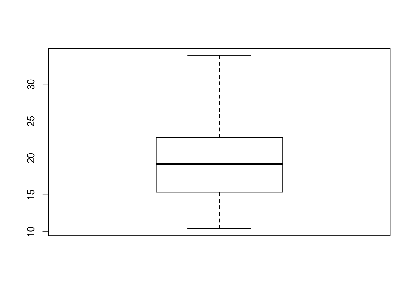
We saw already how to create a boxplot in R. Let’s try it on the mpg variable from the mtcars dataset:
boxplot(mtcars$mpg)
Recall that the dollar sign $ can be used to access individual variables in a data frame, so mtcars$mpg is how I get the value of the mpg variable.
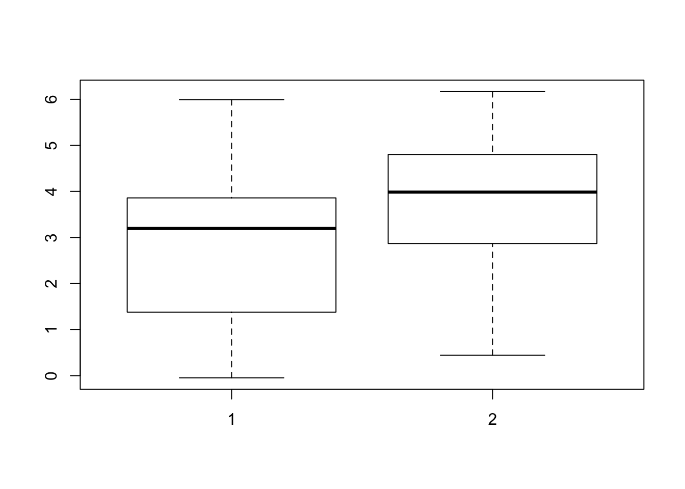
This particular plot gives us some sense of the shape of the mpg values, but boxplots really come into their own when comparing different groups. There are two ways this can be done: by having the values for each group in a different argument, for example Xs and Ys from the first exercise:
boxplot(X, Y)
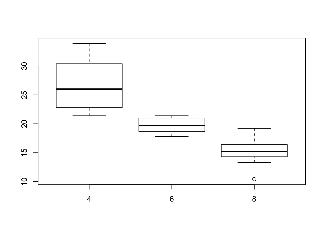
However, we can also use a more concise notation when the grouping variable is already part of the dataset. With mtcars, we have such a grouping variable in cyl, indicating the number of cylinders in the engine. In this case, we can write:
boxplot(mpg ~ cyl, data = mtcars)